Advanced LLM Compression: A Deep Dive into REAP

The arms race in artificial intelligence is governed by scaling laws and the Chinchilla coefficient (where parameter size multiplied by 20 dictates the required pre-training tokens). Labs are initializing models with more weights and training them on vastly larger datasets to achieve emergent intelligence. However, this brute-force approach has collided with a severe hardware reality: memory bandwidth and VRAM capacity.

With enterprise-grade VRAM hovering around $500 per GB and global SRAM/DRAM shortages capping physical expansion, running frontier open-weight models locally requires serious architectural optimization.

This post explores the mechanics of Router-Weighted Activation Pruning (REAP), a highly effective compression technique for Mixture of Experts (MoE) architectures, and how it enables the local execution of massive parameters on accessible hardware.

The Problem with Scaling Laws and MoE Architectures

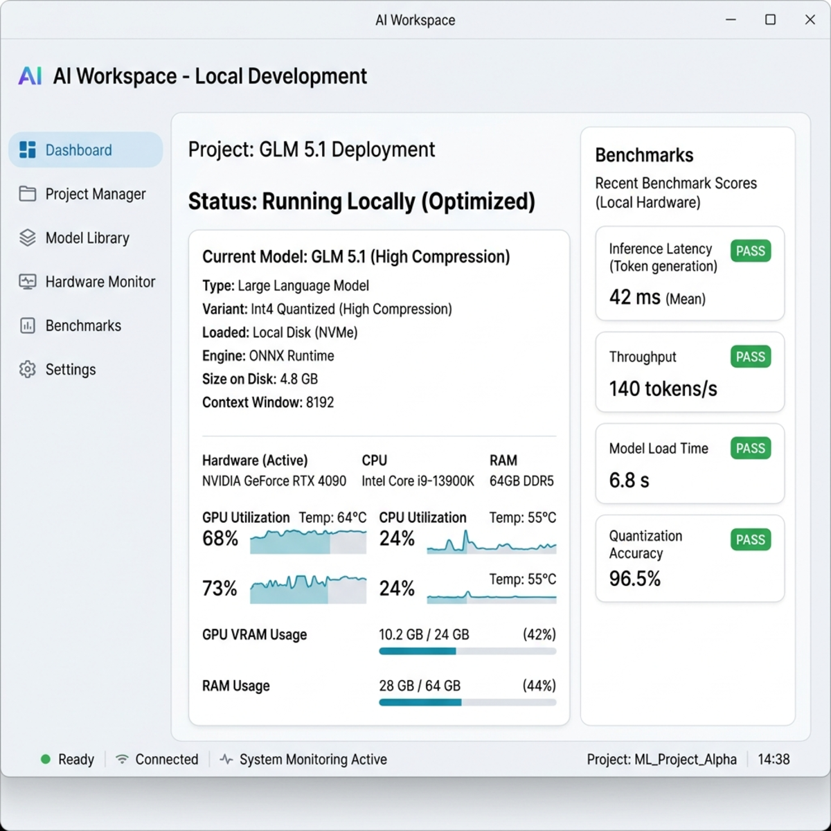
Models like GLM 5.1 (478 billion parameters) dictate the bleeding edge of open-source capabilities. Uncompressed, this model requires roughly 1.5 TB of VRAM just to load the weights, and closer to 2 TB to account for the KV cache during active inference.

To mitigate inference costs, modern architectures utilize the Mixture of Experts (MoE) design. Instead of activating the entire network for every prompt, tokens pass through a routing mechanism that directs them to specific expert neural networks. Typically, only about 8% of the model activates per token. This vastly improves generation speed and lowers electricity consumption. However, the model still requires the entire massive weight file to be loaded into VRAM.

Enter REAP: Router-Weighted Activation Pruning

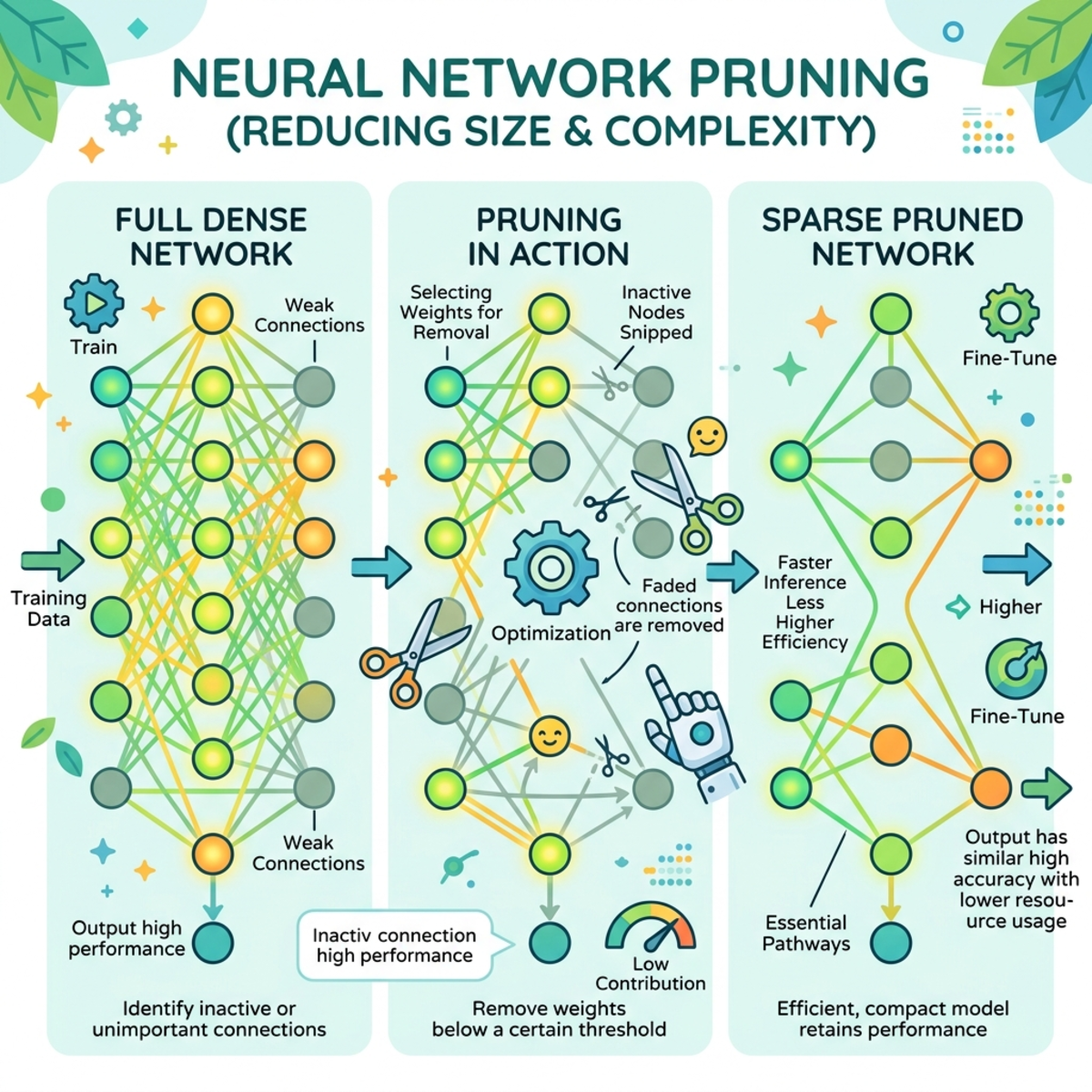
REAP is a compression methodology designed exclusively for MoE models. Unlike generic pruning, which might blindly chop parameters, REAP maps the exact neural pathways that matter for your specific use case.

The process relies on a calibration dataset. If your primary goal is agentic engineering or terminal-based development (e.g., integrating with LM Studio, the Codex app, or Figma MCP integrations), you feed the model a dataset consisting of code documentation, system prompts, and structured output examples.

As the model processes this data, it generates saliency heat maps. You can visualize which specific experts (out of potentially hundreds of thousands) are actively lighting up to handle tasks like tool calling or JSON generation. Once the critical pathways are mapped, you can aggressively prune the dead weight:

• Targeted Preservation: Keep the experts that handle your specific workloads (e.g., Python, UI design, structured logic).
• Targeted Lobotomy: Feed the model prompts designed to trigger refusals (e.g., “I am just an AI assistant…”). Map those active experts and cut them out to effectively bypass system-level guardrails.
• Expert Resizing: Retain the most highly active experts at full size while shrinking the less critical ones.

Pruning vs. Quantization

It is vital to distinguish between pruning and quantization, as they address VRAM limitations from completely different angles:

• Pruning (REAP): Physically removes experts from the MoE architecture. The model loses access to whatever data was stored in those weights.
• Quantization: Reduces the numerical precision of the weights (e.g., converting 16-bit floating points to 4-bit representations). It relies on the fact that the ratios between weights matter more than the absolute precision.

These methods synergize. By applying maximum recommended REAP alongside an aggressive quantization format (like Nvidia’s NVFP4 4-bit quantization), it is possible to achieve a 12.5% total model size compression without severe performance degradation on targeted tasks.

In practice, this allows you to run a model like GLM 5.1 (478B) locally on roughly 370 GB of VRAM, bringing frontier capabilities directly into local server racks.

The Big Pruned Model vs. The Small Native Model

A common question in local LLM optimization is whether it is better to prune a massive 100B model down to 25B or simply run a native 25B model. The answer lies in the pre-training data.

Metric	Pruned Massive Model (e.g., 100B pruned to 25B)	Native Small Model (e.g., 25B)
Pre-training Data Seen	Massive (Guided by Chinchilla coefficient, e.g., 2 Trillion+ tokens)	Limited (Hit a mathematical wall around 500 Billion tokens)
Base Intelligence	Exceptionally high; benefits from larger lab budgets and superior engineering.	Moderate; constrained by the hard limits of its parameter size.
Agentic Capability	Highly resilient in complex loops, structured reasoning, and multi-tool calling.	Prone to overthinking, looping errors, and workflow degradation.

Even when 75% of a massive model is removed, the remaining 25% contains higher-quality, deeply optimized intelligence derived from a vastly larger training run.

Evaluation, Benchmarks, and Model Surgery

Amateur pruning often destroys a model’s ability to execute precise tasks like tool calling. Following a REAP compression, rigorous evaluation is mandatory. You must run standardized benchmarks (SweBench verified, HumanEval, Terminal Bench) to quantify the degradation.

If an evaluation reveals that the pruned model is failing at structured outputs, you can perform advanced model surgery:

1. Re-inject previously pruned experts back into the architecture.
2. Take higher-precision (16-bit) neurons from the original model for the specific tool-calling experts and graft them onto your quantized/pruned model to restore accuracy.

Advanced Optimization Tactics

To maximize hardware efficiency and reduce compute overhead during the compression phase, several advanced workflows can be deployed:

• Pre-Quantized Pruning: Running REAP on a full-precision model requires massive compute. You can apply quantization first, shrinking the model by 75%, and then run the REAP calibration on significantly cheaper hardware setups to lower VRAM overhead.
• Shared Observation Files: The saliency mapping process generates observation/text files. Because the underlying MoE architecture is identical across instances, these files can be shared across the community. You can apply pre-mapped expert routing without spending the repetitive GPU cycles to compute it yourself.
• Predictive Routing (The Future): Because ~20% of a model handles 95% of standard prompts, the next phase of optimization involves training a secondary, tiny predictive model. This model intercepts the prompt, predicts which experts will be needed, and dynamically shifts those experts from SSD to RAM to VRAM just-in-time. Theoretically, this could reduce the active hardware footprint to as little as 5% of the original model size without sacrificing intelligence.