Why Fast LLMs Still Make Slow Agents: The Agentic Bottleneck

Writer

A model can generate text at more than 1,000 tokens per second and still sit inside an agent that takes minutes to finish a task.
That is not a contradiction. Token-generation speed and agent-completion speed measure different systems.
A chat completion is mostly one inference transaction. An agent is a distributed workflow: it repeatedly invokes a model, calls tools, waits for external systems, expands its context, recovers from errors, and decides what to do next. Every loop adds another opportunity for latency—and many of those delays occur outside the model.
This is the agentic bottleneck: the gap between the speed of an individual model invocation and the wall-clock time required to complete a multi-step task.
The bottleneck is not located in one component. It emerges across five layers:
- Application: tools and external systems introduce variable waiting time.
- Inference: every turn may require processing an increasingly large context.
- Memory and scheduling: agent pauses make KV-cache retention difficult.
- Orchestration: sequential plans, unnecessary steps, and retries extend the critical path.
- Model behavior: unreliable tool selection and malformed arguments create avoidable loops.
The practical lesson is simple: a faster model helps, but it cannot make the rest of the workflow disappear.
Tokens per second is not task completion time
High-speed inference is real. Cerebras reported 1,800 output tokens per second for Llama 3.1 8B and 450 tokens per second for Llama 3.1 70B in 2024. In February 2026, OpenAI introduced GPT-5.3-Codex-Spark as a research preview capable of more than 1,000 tokens per second on Cerebras hardware.1 2
Those numbers describe sampling speed under particular model, hardware, and workload conditions. They do not describe how long an agent takes to complete a job.
A useful approximation is:
OpenAI used a similar decomposition when describing Codex-Spark task duration: output generation, prefill, tool execution, and network overhead all contribute to elapsed time.2
This distinction matters because optimizing only tokens per second attacks just one term—and often not the largest one.
1. The application layer: agents wait on the world
A conventional completion follows a relatively short path:
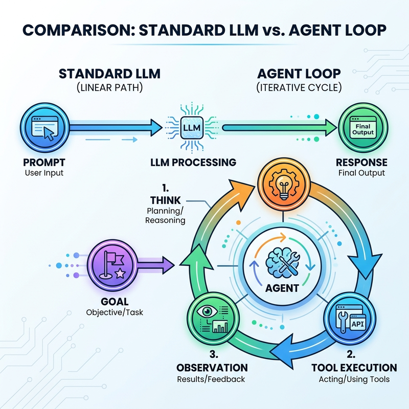
ReAct formalized this pattern by interleaving reasoning and actions, allowing a model to use observations from an external environment to update its next step.3
The loop is powerful precisely because it connects the model to systems beyond its parameters. It is also why latency becomes unpredictable. A tool call may involve:
- a database query;
- a web request;
- repository search or code execution;
- an MCP server;
- a file transfer;
- a SaaS API with its own rate limits;
- a human approval step;
- or another agent.
The model may produce a function call in milliseconds, but the called system can take milliseconds, seconds, or minutes. If the next decision depends on that result, the workflow cannot advance until the observation returns.
Key point: Agents are not always model-bound. They are frequently critical-path-bound by the slowest required inference step, tool call, dependency, or retry.
Tool latency does not always dominate. A reasoning-heavy agent using fast local tools may spend most of its time in model inference. A retrieval agent with slow back-end services may spend most of its time waiting on I/O. The correct diagnosis therefore requires traces, not assumptions.
Latency compounds across turns
Even modest delays become painful when repeated sequentially. Suppose an agent performs 12 model turns and 8 required tool calls:
A two-second delay is tolerable once. Repeating it across a long dependency chain turns it into a user-visible pause.
That is why an agent should be evaluated using end-to-end job completion time, not only time to first token or output tokens per second.
2. The inference layer: every observation can trigger another prefill
Agent loops do not merely generate more output tokens. They repeatedly send an expanding history back into the model:
Before generating the next token, the serving system processes this input during prefill and constructs attention state for it. As the trajectory grows, repeated prefill can become a substantial part of latency—especially when each turn produces only a short tool call after reading a large context.
This creates an important asymmetry:
| Phase | What it does | Typical pressure |
|---|---|---|
| Prefill | Processes the prompt or newly supplied context and builds attention state | Compute-intensive, especially for long inputs |
| Decode | Generates output one token at a time using the existing state | Often constrained by memory bandwidth and per-token scheduling |
| Tool wait | Pauses model progress while an external action runs | Controlled by the application, network, and target system |
A high decode rate does not eliminate long prefill, repeated prefill, or tool waiting. For many agent turns, the model reads thousands of input tokens only to emit a small structured action. In those cases, improving input processing and context reuse can matter more than increasing output-token speed.
3. The memory layer: the KV cache meets an interrupted workload
During inference, transformer serving systems maintain a key-value cache, or KV cache, containing attention states for previously processed tokens. Reusing those states avoids recomputing the entire prefix during generation.
Agent workloads make KV-cache management harder because they alternate between bursts of inference and pauses for tools:
During the pause, the session’s cached state may still be valuable—but GPU high-bandwidth memory is scarce. A serving system must decide whether to:
- retain the cache on the accelerator;
- evict it and recompute the context later;
- offload it to host memory or another storage tier and reload it when needed; or
- preserve only selected reusable prefixes.
The original intuition that a GPU must sit completely idle while holding one agent’s cache is too simplistic. Production servers normally batch and schedule many requests, so compute can serve other work. The real problem is that a paused session’s cache occupies memory capacity, which can reduce concurrency or force eviction. If evicted state is needed again, the system pays a reload or recomputation cost.
Retain, evict, offload—or recompute?
There is no universally optimal policy.
- Retain on GPU: Fastest resumption, but consumes the most expensive memory while the tool runs.
- Evict and recompute: Frees memory immediately, but repeats prefill work when the agent resumes.
- Offload and reload: Preserves reusable state outside GPU memory, but adds data-transfer latency and bandwidth demand.
- Use a time-to-live policy: Keep likely-to-return sessions temporarily, then evict them if the pause lasts too long.
The 2026 Continuum research system focuses directly on this problem. It assigns a time-to-live to KV state for agent requests, weighing the cost of retention against reload, recomputation, and queueing. Its authors report more than an 8× improvement in average job completion time in their evaluated agent workloads, but this remains a research result tied to their workloads, models, and implementation—not a universal production guarantee.4
Mental model: Treat GPU-resident KV cache as a hotel room near the airport. Keeping the room makes the return journey fast, but blocks another guest. Checking out frees capacity, but returning requires a new check-in. Offloading stores the luggage elsewhere; whether that helps depends on how quickly it can be retrieved.
Offloading moves the bottleneck; it does not erase it
KV-cache offloading can reduce recomputation and relieve HBM pressure, but cached state can be large. Moving it between accelerators, host memory, pooled memory, or storage consumes bandwidth and adds latency. If reloading takes longer than recomputing, offloading loses.
The design question is therefore not simply Can the cache be offloaded? It is:
Can useful state be moved and restored quickly enough to beat recomputation without congesting the data path?
This is why practical systems care about fast interconnects, cache-aware routing, tiered memory, and workload-specific eviction policies.
Prompt caching is related—but not the same thing
Anthropic’s prompt caching allows repeated prompt prefixes to be reused, with a five-minute default lifetime and an optional one-hour duration at additional cost.5
That feature is useful evidence that prefix reuse matters for long, repetitive, multi-turn workloads. However, an API-level prompt cache should not be presented as proof of a particular physical KV-offloading architecture. The public behavior tells us that reusable prefixes can reduce repeated processing; it does not reveal exactly how the provider stores or moves internal attention state.
This distinction prevents an implementation inference from being mistaken for a documented product fact.
4. The serving layer: prefill and decode want different things
Prefill and decode have different computational profiles. Serving both phases in the same worker pool is operationally simple, but one phase can interfere with the latency of the other.
Disaggregated inference separates prefill and decode onto different workers or pools. DistServe, presented at OSDI 2024, assigns the phases to different GPUs and coordinates resource allocation for time-to-first-token and time-per-output-token objectives. In its evaluated workloads, DistServe reported up to 7.4× more requests served under latency constraints, or up to 12.6× tighter service-level objectives compared with the evaluated baselines.6
A simplified topology looks like this:
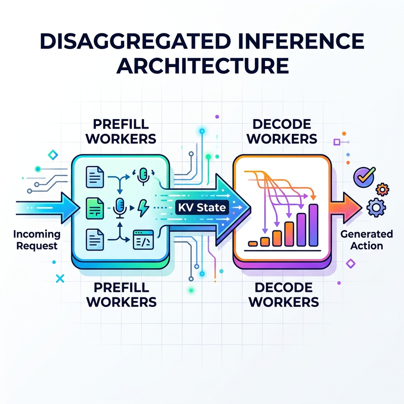
This separation can improve utilization and allow each pool to be tuned differently. But it also creates a new dependency: KV state must cross the network quickly enough that the transfer does not cancel the benefit.
Disaggregation is therefore a trade-off, not free acceleration:
| Potential benefit | New cost or risk |
|---|---|
| Isolate prefill and decode interference | Transfer KV state between pools |
| Scale the two phases independently | Operate a more complex distributed system |
| Tune hardware and scheduling per phase | Depend more heavily on network bandwidth and locality |
| Improve fleet utilization under suitable load | Gain little at small scale or under the wrong traffic shape |
This is mainly a fleet-level optimization. A single-user local workstation does not have the same multi-tenant scheduling problem, so large-scale disaggregation and cache eviction policies may provide less value than simple locality.
DualPath: using both sides of the storage network
Disaggregation can expose another bottleneck. In a conventional prefill/decode split, externally stored KV state is commonly loaded through the prefill workers. Under long, multi-turn agent workloads, that can saturate the storage-facing network interfaces on the prefill side while equivalent interfaces on decode workers remain underused.
DualPath, a 2026 research system from authors affiliated with Peking University, Tsinghua University, and DeepSeek-AI, adds a second loading route:
A global scheduler chooses between the paths to spread storage traffic across the cluster. The paper reports up to 1.87× higher offline throughput and an average 1.96× improvement in online serving throughput without violating the evaluated service-level objectives.7
This result corrects an important misconception: DualPath is not a generic name for moving cache between storage tiers, and disaggregated inference does not inherently reduce throughput. DualPath addresses a specific storage-bandwidth imbalance that can appear when agent contexts are repeatedly restored in a prefill/decode-disaggregated system. Its value depends on large reusable caches, external storage, suitable RDMA connectivity, and enough traffic to expose the imbalance.
5. The orchestration layer: the critical path is often sequential
Even perfect inference infrastructure cannot repair an inefficient plan.
Many agents use a ReAct-like loop in which each observation determines the next action. That dependency makes the workflow inherently sequential:
If step 7 depends on the result of step 6, they cannot run concurrently. The only ways to shorten that path are to:
- make each required step faster;
- reduce the number of required steps;
- avoid failures and retries; or
- identify independent work that can safely overlap.
Parallelism helps only where dependencies allow it
An orchestrator may be able to run independent operations concurrently:
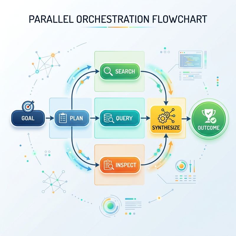
That can reduce elapsed time from roughly the sum of branch durations toward the duration of the slowest branch, plus coordination overhead.
But parallelism is not automatically better. It can:
- duplicate work;
- increase token and tool consumption;
- create conflicting state changes;
- overload downstream systems;
- and add synthesis overhead.
The best strategy is not “use more sub-agents.” It is parallelize independent, valuable work while keeping state-mutating actions controlled and avoiding speculative fan-out with low expected value.
The harness can create its own latency
The agent harness includes much more than the visible loop:
- system instructions and tool schemas;
- context construction and truncation;
- model routing;
- tool selection and execution;
- validation and repair;
- retry and timeout policy;
- persistence and checkpointing;
- tracing and policy enforcement.
Poor harness design adds unnecessary model calls, oversized prompts, repeated serialization, redundant tool discovery, and broad retries. These costs compound on every turn.
A useful ablation method is to hold the model constant while changing the harness, then hold the harness constant while changing the model. That separates model capability from orchestration quality more reliably than comparing two complete products and attributing the difference to one component.
6. The model layer: tool-use reliability is a performance feature
A model can be strong at general reasoning and still be inefficient as an agent if it is unreliable at tool use.
A common failure sequence looks like this:
- The model selects the wrong tool or invents an argument.
- The tool rejects the request.
- The harness returns the error to the model.
- The model retries with another malformed call.
- The loop consumes more input, output, time, and tool capacity.
This is not merely a quality problem. It is latency amplification.
Tool-use post-training and structured-output techniques aim to improve behaviors such as:
- recognizing when a tool is necessary;
- selecting the correct function;
- supplying valid arguments;
- respecting schemas and types;
- using multiple tools in the correct order;
- declining irrelevant tools;
- and recovering efficiently from errors.
The Berkeley Function Calling Leaderboard evaluates function- and tool-calling behavior. Its scope has expanded beyond simple calls to include multiple and parallel calls, relevance detection, multi-turn interactions, and broader agentic evaluations.8
BFCL is useful evidence, but it is not a complete agent benchmark. A high score does not guarantee low end-to-end latency, good planning over long horizons, safe side effects, or success with a company’s private tools. Production evaluation still needs task-level traces and domain-specific tests.
7. Agent workloads rebalance the surrounding infrastructure
The original argument extends below model serving into overall system design. A single-pass generation workload can appear GPU-centric because most visible work is prompt processing and token generation. An agentic job repeatedly crosses the boundary between accelerator compute and the rest of the platform.
That increases the importance of:
- CPUs, for orchestration, tool processes, serialization, validation, scheduling, and application logic;
- Memory and storage, for accumulated context, tool results, checkpoints, artifacts, and externalized KV state;
- Networking, for model calls, remote tools, databases, storage traffic, and inter-worker KV transfer;
- Power delivery and cooling, for a heterogeneous workload whose components may become active at different points in the loop.
This should not be translated into a universal CPU-to-GPU or power-allocation ratio. The correct blend depends on the agent, model placement, tool topology, concurrency, context length, and cache policy. The defensible conclusion is narrower: agentic systems increase the importance of the infrastructure surrounding the accelerator, so capacity planning cannot be based on GPU throughput alone.9
The workload can also be bursty. Model inference may drive the accelerators, followed by CPU-heavy orchestration, network transfers, storage access, or external waiting. At fleet scale, that shifts the design question from “How many tokens can this GPU generate?” to “Can the entire heterogeneous system sustain the agent’s sequence of compute, movement, waiting, and resumption?”
8. Local agents face a different version of the problem
The large-scale agentic bottleneck is dominated by fleet scheduling, concurrency, memory pressure, and distributed data movement. A local agent running for one user has a different constraint profile.
The same machine may need to support:
- model inference on the GPU or unified accelerator;
- orchestration and tool processes on the CPU;
- large contexts in GPU or system memory;
- repository scanning and caching on local storage;
- containers, compilers, browsers, and databases;
- and cooling and power delivery under sustained load.
Raw accelerator speed still does not guarantee a fast agent. A coding agent can be blocked by compilation, tests, filesystem scans, insufficient RAM, storage contention, or an overloaded CPU even when model decoding is fast.
The optimization priority also changes. With no competing tenants, keeping state resident may be reasonable. Complex remote offloading may add more overhead than it removes. Local systems benefit first from balanced hardware, context discipline, fast tools, and instrumentation that identifies the actual idle periods.
Measuring the agentic bottleneck
Optimizing agents requires a trace that follows the entire task, not a dashboard containing only model tokens.
At minimum, capture:
| Metric | What it reveals |
|---|---|
| End-to-end task time | The duration users actually experience |
| Time to first token (TTFT) | Prompt processing, queueing, and initial inference delay |
| Time per output token (TPOT) | Decode responsiveness |
| Prefill tokens and duration per turn | Cost of repeatedly processing growing context |
| Tool duration by tool and percentile | External critical-path delays and tail latency |
| Model turns per completed task | Planning efficiency |
| Retry and invalid-call rate | Latency caused by tool-use failures |
| Cache hit, eviction, reload, and recomputation rates | Whether context reuse is helping |
| Queueing time | Capacity and scheduling pressure |
| Parallel branch utilization | Whether concurrency shortens the critical path |
The most revealing visualization is usually a distributed timeline:
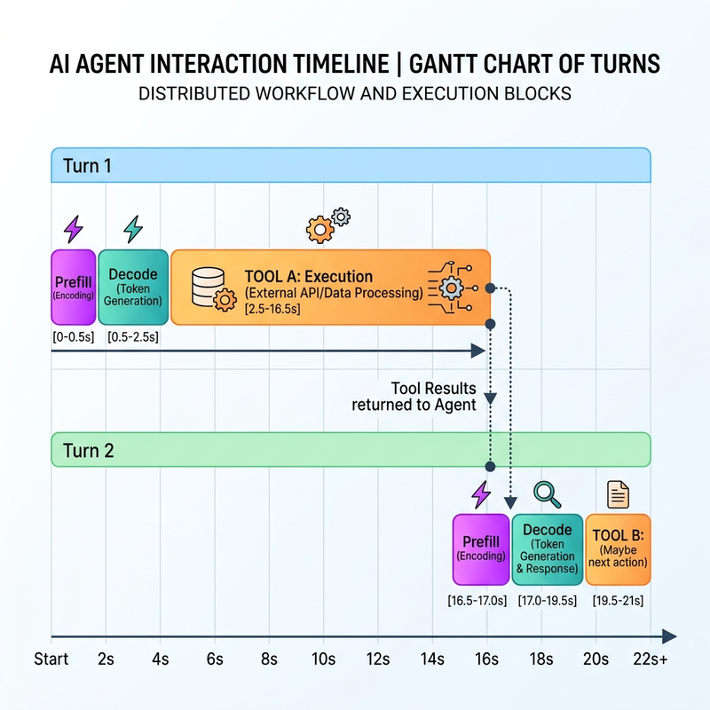
Once the time is visible, optimization becomes less mysterious.
A practical optimization order
There is no single cure, but there is a sensible sequence.
1. Shorten the plan
Reduce unnecessary turns, duplicate searches, repeated validation, and over-broad decomposition. The fastest step is the one the agent does not need to perform.
2. Fix slow and unreliable tools
Measure percentiles, not just averages. Add timeouts, bounded retries, efficient query patterns, result limits, and idempotency where actions can be repeated.
3. Control context growth
Avoid returning huge tool payloads when a compact, faithful result will do. Keep stable instructions and schemas cache-friendly. Summarize old observations carefully without discarding information required for later decisions.
4. Reuse processed prefixes
Use supported prompt caching or server-side prefix/KV reuse where the workload has stable repeated context. Verify actual cache hits rather than assuming configuration is effective.
5. Parallelize only independent work
Start with read-only branches whose results can be combined safely. Protect state-changing actions with ordering, validation, and conflict controls.
6. Improve model–tool fit
Evaluate models on your real schemas, argument distributions, failure modes, and multi-turn tasks. A slightly slower model that avoids retries can finish the job sooner.
7. Optimize serving architecture at scale
When measurements show heavy prefill/decode interference or sustained KV pressure, investigate cache-aware scheduling, offloading, disaggregated prefill/decode, and hardware specialization. These are infrastructure responses to observed workload shapes—not default requirements for every agent.
What each optimization can—and cannot—solve
| Technique | Helps with | Does not eliminate |
|---|---|---|
| Faster decoding | Long generations and model response time | Slow tools, repeated prefill, bad plans |
| Prompt or prefix caching | Repeated processing of stable prefixes | New context, tool waiting, invalid calls |
| KV-cache retention | Fast continuation after short pauses | HBM capacity pressure |
| KV-cache offloading | HBM pressure and avoidable recomputation | Transfer overhead and network limits |
| Prefill/decode disaggregation | Phase interference and fleet specialization | Tool latency and orchestration errors |
| Parallel tools or sub-agents | Independent branches on the critical path | Sequential dependencies |
| Better tool-use training | Invalid calls, retries, and recovery loops | Slow external systems |
| Faster tools | I/O-bound agent steps | Model and scheduling latency |
The deeper architectural shift
Agent workloads change the unit of optimization.
For ordinary generation, the unit is often a request or token. For agents, the meaningful unit is a stateful job that repeatedly crosses boundaries among models, tools, schedulers, networks, memory tiers, and external services.
That shift has three consequences:
- Performance becomes end-to-end. A record token rate can coexist with a slow task.
- State becomes a first-class resource. Context must be retained, reused, moved, summarized, or recomputed across pauses.
- Reliability affects latency. Every incorrect tool call or failed recovery adds another trip around the loop.
The agentic bottleneck is therefore not evidence that agents are inherently doomed to be slow. It is evidence that the architecture is no longer a single inference pipeline.
Conclusion
AI agents feel slow because they force fast probabilistic compute to coordinate with slower, variable, stateful systems.
The delay can come from tool execution, repeated prefill, growing contexts, KV-cache pressure, network transfer, queueing, sequential plans, unnecessary model turns, or invalid function calls. Different workloads produce different combinations, so the solution begins with tracing the full job.
The durable design rule is this:
Optimize the critical path of the agent, not just the token stream of the model.
Faster models remain valuable. But the next generation of responsive agents will also require better tools, smaller plans, stronger function calling, disciplined context management, cache-aware scheduling, and—in sufficiently large serving fleets—carefully designed disaggregated infrastructure.
References
Footnotes
-
Cerebras, “Introducing Cerebras Inference: AI at Instant Speed”, August 27, 2024. ↩
-
OpenAI, “Introducing GPT-5.3-Codex-Spark”, February 12, 2026. ↩ ↩2
-
Shunyu Yao et al., “ReAct: Synergizing Reasoning and Acting in Language Models”, submitted October 6, 2022; ICLR 2023. ↩
-
Hanchen Li et al., “Continuum: Efficient and Robust Multi-Turn LLM Agent Scheduling with KV Cache Time-to-Live”, revised May 25, 2026. ↩
-
Anthropic, “Prompt caching”, Claude Platform documentation, accessed July 20, 2026. ↩
-
Yinmin Zhong et al., “DistServe: Disaggregating Prefill and Decoding for Goodput-optimized Large Language Model Serving”, OSDI 2024. ↩
-
Yongtong Wu et al., “DualPath: Breaking the Storage Bandwidth Bottleneck in Agentic LLM Inference”, revised February 26, 2026. ↩
-
UC Berkeley Gorilla project, “Berkeley Function-Calling Leaderboard V4”, updated April 12, 2026. ↩
-
NVIDIA, “Scaling Agentic AI Factories Through Extreme Co-Design with NVIDIA BlueField”, July 16, 2026. This vendor source is used only to support the general observation that agentic workloads involve GPUs, CPUs, memory, networking, storage, and context movement—not a prescribed hardware ratio. ↩
Read next