Architecting Cost-Effective Agentic Workflows with Three-Tier Routing

The era of AI orchestration is forcing a fundamental shift in how we build and scale enterprise systems. As agentic engineering takes hold, we are moving from single-prompt interactions to autonomous agents that recursively query, plan, and execute. This amplification creates a massive surge in capability — but it also triggers an exponential explosion in token consumption.

In this article, we will talk about one of the critical architectural pivots needed to survive this token economic crisis. By blindly routing every prompt to massive 70-billion+ parameter cloud models, organizations are burning capital, increasing latency, and wasting computational resources.

The solution lies in intelligent orchestration, local large language model (LLM) inference, and a custom routing classifier. This article is the architectural blueprint and a hands-on implementation guide: by the end you will have a complexity-scoring rubric, a working classifier, concrete model and quantization picks per tier, and a step-by-step rollout plan you can run this week.

The Broken Math of Token Economics

In standard development workflows, tokens accumulate rapidly. A seemingly simple request sent to a massive cloud model like Claude Opus 4.7 or GPT-4o incurs unnecessary overhead — you pay frontier-model rates to fix a lint error. The baseline token costs of daily developer tasks add up quickly:

Here is where the math breaks. A single developer prompt rarely stays a single inference call. In an agentic loop, the orchestrator decomposes one request into a plan, spawns sub-agents to gather context, calls tools, critiques its own output, and retries — the AI multiplier effect. One “simple” prompt can fan out into 10–100 model calls.

For a standard 50-person development team, naive cloud inference can run roughly $36,000 per month. Apply a 10x agentic multiplier and you reach $360,000; a 100x multiplier on heavy autonomous workflows pushes you toward $3.6 million. The lesson is not “agents are too expensive” — it is that treating all compute as equal is the expensive part. Most of those fan-out calls are trivial and never needed a frontier model.

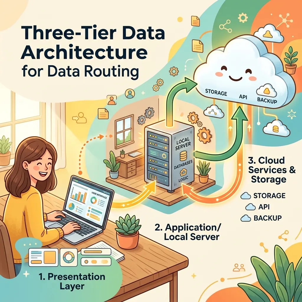
The Three-Tier Inference Architecture

Workload analysis from Claude Sonnet 4.6 traffic suggests that up to 73% of enterprise coding tasks are edge-resolvable, and roughly 34% rank as “simple” (complexity score 1–4). In other words: the majority of your token spend is going to models that are wildly overqualified for the job.

Instead of defaulting to the cloud, route every prompt through a three-tier architecture:

1. Tier 1 — Local Edge Devices (≤ 13B parameters): Code completion, boilerplate, docstrings, simple lint fixes. Runs entirely on the developer’s own NPU/GPU laptop. Cost per token: $0. Target latency: < 200 ms.
2. Tier 2 — On-Premise Workstations / Servers (~30B–120B parameters): Mid-complexity work — multi-file edits, test generation, moderate refactors. Runs on a shared GPU server on your network.
3. Tier 3 — Cloud APIs (> 120B parameters): Reserved for genuinely hard logic — cross-repo refactoring, architectural reasoning, and security/compliance audits where precision is non-negotiable.

By shifting simple and medium tasks to Tier 1 and Tier 2, a 50-person team can process the bulk of its volume — on the order of 1.6 billion tokens — locally at near-zero marginal cost, cutting that $36,000 baseline down to roughly $12,000. The cloud bill becomes a small, deliberate line item instead of the default.

What actually runs on each tier

Theory is cheap; here are concrete, deployable picks (all open-weight examples — swap in your preferred models):

Hardware Optimization and Quantization Strategies

Executing Tier 1 locally means optimizing for two things: memory capacity (can the model even fit?) and memory bandwidth (how fast can you stream weights per token?). Inference on these devices is almost always bandwidth-bound, not compute-bound.

Modern NPUs make this viable. The Snapdragon X2 Elite, for example, delivers up to 80 TOPS (INT8) of NPU compute, supports up to 128 GB of unified LPDDR5X memory, and reaches up to 228 GB/s of memory bandwidth (the mainstream Elite SKUs sit at 152 GB/s; the Extreme variant hits 228 GB/s). That bandwidth — not the TOPS number — is what determines your tokens-per-second on a quantized model.

To fit capable models onto these devices, quantization is mandatory. Moving from 16-bit floating point to reduced-integer formats cuts both the memory footprint and the bandwidth you must stream per token by up to ~50% (FP16 → INT8) and far more at INT4. A practical sizing rule of thumb:

VRAM/RAM needed ≈ (parameters in billions) × (bytes per weight) × 1.2 overhead. A 7B model at Q4_K_M (~0.5 bytes/param effective) needs ≈ 4–5 GB; the same model at FP16 needs ≈ 14 GB.

Match the format to the task’s precision sensitivity:

• Complexity scores 1–6: Integer quantization (INT4/INT8, Q4_K_M/Q8_0) introduces a maximum quality gap of ~5% — invisible for boilerplate and completion. Ideal for Tier 1 edge execution.
• Complexity scores 7+: Precision matters. Numerical or logic-heavy work degrades under aggressive quantization, so keep these in higher precision (FP16/BF16) and route to Tier 2 or Tier 3 to avoid precision collapse.

Building the Orchestrator’s Brain: The Classifier

The core intellectual property of your agentic framework is the Orchestrator’s Classifier — a lightweight, sub-20-millisecond decision unit that sits in front of every prompt. Its only job: score the prompt, pick the tier, and arm a fallback. It must be cheap enough that it never becomes the bottleneck (keep its own overhead under ~50 tokens / 20 ms).

It works in two layers: four static signals computed before routing, plus one runtime signal (the fallback) that watches execution.

The four static signals (computed pre-route):

1. Prompt / context size — Token count and attached file size. Large contexts correlate with harder tasks and push the score up.
2. Abstract Syntax Tree (AST) depth — Parse the referenced code and measure nesting depth of the logic to be modified. Deep, branchy if/then/loop structures signal a need for a larger-parameter model. (The original “Abstract System Tree” is an AST — parse the code, don’t guess.)
3. Cross-file reference count — How many distinct files/modules must be synthesized? Requests spanning many isolated files carry higher entropy and usually need Tier 3.
4. Security & compliance flags — Any prompt touching auth, crypto, secrets, PII, or injection-prone surfaces is force-routed to secure, high-tier processing regardless of its other scores.

Combine these into a single 0–10 complexity score and map it to a tier:

Here is a minimal, readable reference implementation:

import ast, re, time

SECURITY_PATTERN = re.compile(
    r"\b(auth|password|secret|token|crypto|encrypt|jwt|sql|injection|pii)\b",
    re.IGNORECASE,
)

def ast_depth(code: str) -> int:
    """Max nesting depth of the code's AST (0 if unparseable)."""
    try:
        tree = ast.parse(code)
    except SyntaxError:
        return 0
    def depth(node, d=0):
        children = list(ast.iter_child_nodes(node))
        return d if not children else max(depth(c, d + 1) for c in children)
    return depth(tree)

def complexity_score(prompt: str, code: str, file_refs: int) -> int:
    score = 0
    score += min(len(prompt.split()) // 200, 3)   # 1. context size  -> 0..3
    score += min(ast_depth(code) // 3, 3)          # 2. AST depth     -> 0..3
    score += min(file_refs, 3)                     # 3. cross-file    -> 0..3
    if SECURITY_PATTERN.search(prompt + code):     # 4. security flag -> hard bump
        score = max(score, 8)
    return min(score, 10)

def route(prompt: str, code: str = "", file_refs: int = 0) -> dict:
    t0 = time.perf_counter()
    s = complexity_score(prompt, code, file_refs)
    tier = "tier1_edge" if s <= 4 else "tier2_onprem" if s <= 7 else "tier3_cloud"
    return {
        "complexity_score": s,
        "tier": tier,
        "classifier_ms": round((time.perf_counter() - t0) * 1000, 2),
    }

You can express the routing policy as config so non-engineers can tune thresholds without touching code:

# routing.yaml
tiers:
  tier1_edge:
    max_score: 4
    model: "qwen2.5-coder:7b"
    quantization: "Q4_K_M"
    endpoint: "http://localhost:11434" # Ollama
    timeout_ms: 800
  tier2_onprem:
    max_score: 7
    model: "qwen2.5-coder:32b"
    quantization: "Q8_0"
    endpoint: "http://gpu-server.internal:8000" # vLLM
    timeout_ms: 4000
  tier3_cloud:
    max_score: 10
    model: "claude-opus-4-7"
    endpoint: "https://api.anthropic.com"
fallback:
  escalate_on_timeout: true
  escalate_on_low_confidence: true # logprob / self-eval threshold
  max_escalations: 1

A Step-by-Step Rollout Plan

You do not need to build the whole stack on day one. Stage it:

1. Audit your logs (Week 1). Export the last two weeks of AI coding requests. Score each one with the rubric above (run the complexity_score function over them in batch). You now know your real distribution — most teams find 60–75% land at score ≤ 4.
2. Stand up Tier 1 (Week 1–2). Install Ollama or LM Studio on developer machines, pull a 7B coder model at Q4_K_M, and point your IDE/agent at the local endpoint for score-≤4 traffic only.
3. Stand up Tier 2 (Week 2–3). Deploy a 32B+ model on a shared GPU box with vLLM. Route scores 5–7 there.
4. Wire the classifier + fallback (Week 3). Put the route() function in front of every call, load routing.yaml, and enable timeout/low-confidence escalation.
5. Measure, then tighten (ongoing). Track four numbers per tier: % of traffic, $ per 1k tokens, p50/p95 latency, and fallback (escalation) rate. If a tier’s fallback rate creeps above ~10%, your threshold is too aggressive — nudge it down. If it’s near 0%, you can push more traffic local.

A simple observability table is enough to start:

The Call to Action

Stop routing your basic docstrings to 70-billion parameter models. The competitive advantage in enterprise AI no longer lies in merely having access to foundational models — it lies in how intelligently you orchestrate them.

Strategic advice for developers and enterprises: build the classifier as proprietary IP. It encodes your codebase’s complexity distribution, your security surface, and your cost tolerance — and no vendor can sell you that.

Start this week: audit your request logs, score them with the rubric, stand up a single Tier 1 model with Ollama, wire in the classifier and fallback, then watch your latency drop and your cloud bill shrink. The hardest part is the first ollama pull — everything after that is tuning thresholds.